神经网络解常微分方程
解方程:
1
2
3
4
5
import torchimport torch.nn as nnfrom torch.autograd import Functionfrom matplotlib import pyplot as plt%matplotlib inline
1
2
3
4
5
6
7
8
9
10
11
12
13
14
class NN (nn.Module): def __init__ (self ): super (NN, self).__init__() self.input_layer = nn.Linear(1 , 20 ) self.hidden_layer = nn.ModuleList([nn.Linear(20 , 20 ) for _ in range (4 )]) self.output_layer = nn.Linear(20 , 1 ) self.act = nn.Tanh() def forward (self, x ): o = self.act(self.input_layer(x)) for _, hl in enumerate (self.hidden_layer): o = self.act(hl(o)) out = self.output_layer(o) return out
1 x = torch.linspace(0 , 2 , 2000 ,requires_grad=True ).unsqueeze(-1 )
1
2
3
net = NN() loss_fn = nn.MSELoss(reduction='mean' ) optimizer = torch.optim.Adam(net.parameters(), lr=0.001 )
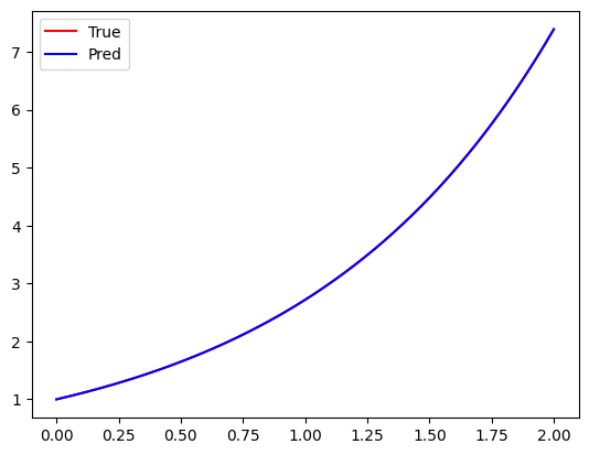
$f(x)$在此是用神经网络NN进行逼近,则$f’(x)$是神经网络的输出对x的导数
1
2
3
4
5
6
7
8
9
10
11
12
13
14
15
16
17
18
19
20
21
22
23
24
25
26
27
28
for epoch in range (1000 ): y_0 = net(torch.zeros(1 )) f = net(x) pf, = torch.autograd.grad(f, x, grad_outputs=torch.ones_like(net(x)), create_graph=True ) optimizer.zero_grad() Mse1 = loss_fn(f, pf) Mse2 = loss_fn(y_0, torch.ones(1 )) loss = Mse1 + Mse2 loss.backward() optimizer.step() if epoch % 200 == 0 : print ("epoch:{}, loss:{}" .format (epoch, loss.item())) y = torch.exp(x) y1 = net(x) plt.plot(x.detach().numpy(), y.detach().numpy(), c='red' , label='True' ) plt.plot(x.detach().numpy(), y1.detach().numpy(), c='blue' , label='Pred' ) plt.legend(loc='best' ) plt.show()
epoch:0, loss:1.452800989151001
epoch:200, loss:0.09077981114387512
epoch:400, loss:0.0009344415157102048
epoch:600, loss:0.0003904764889739454
epoch:800, loss:0.0001252157671842724